PACE v2.0 Documentation
Table of contents
Introduction
ICCT’s Projection of Aviation Climate Effects (PACE) model is a global aviation climate impact model covering commercial passenger and cargo operations. Version 2.0 of the model expanded upon the CO2 focused version 1.0 to capture all known climate pollutants from aviation. The model estimates well-to-wake greenhouse gas emissions and short-lived climate pollutant emissions in future years under different technology pathways. PACE can be used to provide policymakers with insights into actions needed to meet specific climate budgets.
The model uses 2023 activity and emission data from ICCT’s Jet and Turboprop Simulations for Trajectory-based Emissions and Meteorological Effects (JETSTREAM) model as its baseline. The mitigation levers include fuel efficiency improvement, use of sustainable aviation fuels (SAF), fuel hydrotreating, introduction of zero-emission planes (hydrogen and electric), introduction of engines with lower NOx and PM emissions, contrail avoidance maneuvers, demand reduction in response to higher fuel prices, and modal shift to high-speed rail. The model iterates through each analysis year; the changes in traffic, energy, and emissions in one year will affect the modelled outcome of the next.
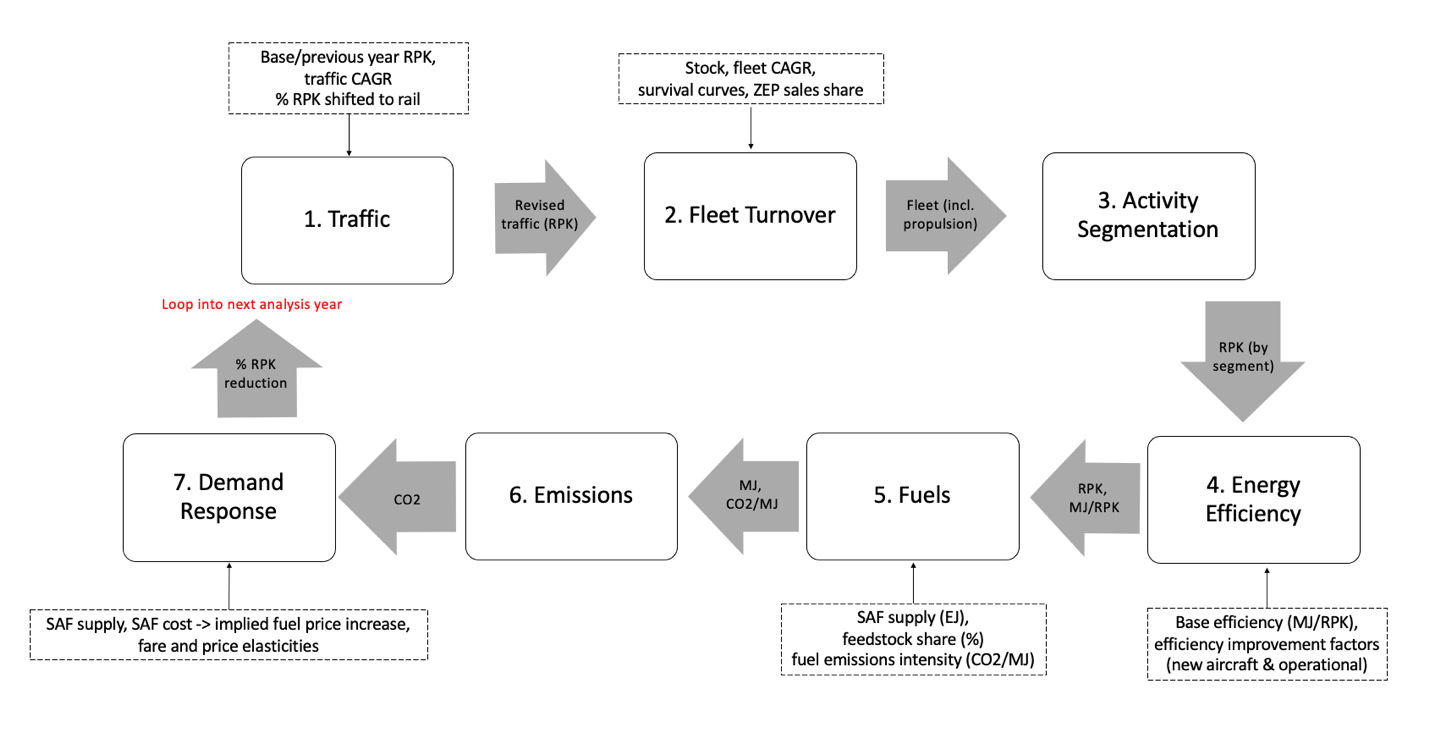
Figure 1. Model flow chart for each analysis year.
It is worth noting that the model treats SAF supply and cost as exogenous variables. The change in traffic growth or fuel efficiency does not affect the amount of SAFs in the system.
This documentation describes the inputs, calculations, and outputs of each module. There are two types of inputs: default inputs that enable baseline model runs, and user-specific assumptions for various modeling scenarios. The 2.0 version of the model was used to model 2020-2050 emissions and contrail-induced effective radiative forcing for ICCT’s “Vision 2050: the Potential of Climate Neutral Growth” report. The “scenario inputs” section describes the specific inputs used for this project.
In addition, all input data are structured in the tidy data format. Every column is a variable. Every row is an observation. Preparing data in such a format is crucial to using the model.
Acknowledgments
PACE was first developed in 2022 by Xinyi Sola Zheng, Jayant Mukhopadhaya, and Erik Pronk. In 2025, v2.0 was developed by Xinyi Sola Zheng and Jayant Mukhopadhaya.
Modules
The PACE model performs analysis on the level of operational segment. Figure 1 shows how we define segments. We used ICAO’s region definition to group traffic into region pairs. There are a total of 10 region designations and 84 valid region pairs (i.e., those with direct flights in between) in 2023, based on ICCT’s inventory. We break down the operations within each region pair based on trip destination (domestic vs. international), aircraft type, and distance band, which results in 1,550 unique segments globally. These will be referred to simply as “segments” for the rest of this document. All the traffic segments are also repeated for each demand segment – passenger, belly freight, and dedicated freight – to allow differentiated inputs. Note that only intra-region segments will have a domestic sub-segment, such as North America-North America, China-China, and so on.
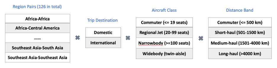
Figure 2. PACE model operational segments.
All future year emissions and climate impacts are computed using the base-year fuel efficiency \((\frac{gCO_{2}}{RTK})\) of each segment from JESTREAM inventory and the fuel intensity or fuel emission intensity reduction factors associated with each mitigation lever. JETSTREAM integrates ADS-B flight trajectories, meteorological data, aircraft performance and contrail process models, and airline operational data to estimate fuel burn, carbon dioxide (CO₂), nitrogen oxides (NOₓ), particulate matter (PM), contrail cirrus formation, and other pollutants from both cruise and landing–takeoff (LTO) operations. The base-year efficiency inputs also differentiate between passenger, belly freight, and dedicated freight, as mitigation levers are not always applied to passenger and cargo operation at the same rate.
1. Traffic
The Traffic Module handles traffic growth, demand response to ticket price increase, and modal shift to rail for relevant segments.
In the first analysis year, the model takes in base-year revenue tonne-kilometer (RTK) data broken down by segment, which come from ICCT’s JETSTREAM model. The model then matches the compound annual growth rates (CAGR) from ICAO’s traffic forecast to the base-year RPK data based on region pair. Table 1 shows the global average growth rates over the modelled time period. The Central Case rates are used by default.
Table 1. Traffic annual growth rates.
| Low | Central | High |
|---|---|---|
Passenger: +2.8% RTK p.a., 2023-2050 |
Passenger: +3.4% RTK p.a., 2023-2050 |
Passenger: +3.7% RTK p.a., 2023-2050 |
Freight: +3.1% FTK p.a., 2023-2050 |
Freight: +3.6% FTK p.a., 2023-2050 |
Freight: +3.9% FTK p.a., 2023-2050 |
Since belly freight is carried on passenger aircraft, its volume is determined by passenger traffic growth. The freight growth rate is applied to dedicated freighter operations only. We also assume that no belly freight is carried on zero-emission aircraft and none of the dedicated freighters are zero-emission aircraft.
In all the following analysis years, the model adjusts each segment’s CAGR based on the percentages of revenue tonne-kilometer (RTK) reduction from ticket price increase in the previous year. These percentages of reduction are calculated in the Demand Module (see Section 7). For analysis years after 2030, when modal shift inputs are given, percentages of traffic shifted to rail are applied to relevant segments. Due to a lack of granular freight pricing data, the model does not incorporate demand response mechanism for dedicated freight.
After adjusting CAGR based on demand reduction rates, the model applies the CAGR onto previous year (Y1)’s RTK by segment (S).
\[\text{RTK}_{S,y2} = RTK_{S,y1}*\left( 1 - RTK_{\text{demand reduction},S,y1} (\%)\right)*(1 + CAGR_{S,y1})\]The overall change in RTK is retained to inform the fleet growth calculation in the Turnover Module (see Section 2). The model also stores the adjusted RTK and CAGR of each segment for demand response calculations later.
2. Turnover
For each aircraft class analyzed, the Turnover Module calculates the fleet growth, ages all aircraft by one year, determines age 0 stock, and integrates ZEPs into age 0 stock based on expected sales shares.
Stock turnover
The overall fleet growth is assumed to be consistent with overall RTK growth. However, the growth of each aircraft class is differentiated. The model takes in annual fleet growth rates for each aircraft class based on industry forecasts. Every year, the model scales these growth rates up or down to match the overall fleet CAGR with the traffic CAGR.
The stock turnover function first takes in the fleet CAGR by aircraft class to calculate the total fleet size for each class. The function then adds one year of age to each row of the “stock by age” data and applies the survival rate matched from year-over-year survival curves. These curves are characterized by a Weibull distribution function, and they represent the fraction of vehicles surviving from one year to the next. ICCT developed these curves as part of an unpublished consultant report to Argonne National Laboratory in 2011. The fleet broken down by age is given for the base year. In this case, for each aircraft type (T), the vehicle stock in a calendar year (CY) of a given delivery year (DY) is calculated as:
\[\text{Stock}_{T,CY,DY} = Stock_{T,CY - 1,DY}*Survival_{T}*(CY - DY)\]Age 0 stock of each class represents estimated new aircraft delivery that year to both replace retired aircraft and to satisfy additional demand. It is set to the gap between the projected fleet size needed to support the traffic volume that year and the number of survived aircraft from the previous year. The age 0 stock (i.e., new sales) is then broken down by propulsion, based on the sales share of hydrogen and electric aircraft in that year, which are user inputs.
\[\text{Stoc}k_{T,\text{CY},\text{DY}} = ProjectedFleetSize_{T,\text{CY}} - \sum_{}^{}{\text{Stoc}k_{T,CY}}\]Zero emission planes (ZEPs)
The model allows for specification of multiple zero-emission aircraft with varying payload and range capability. The introduction year and sales share of these aircraft is input into the model as well. The stock of zero-emission aircraft is limited by the maximum percentage of RTKs they can replace. ICCT’s paper on hydrogen-powered aircraft presents the method for determining the replaceable market for such aircraft. This replaceable market is calculated as a preprocessing step and is dependent on the payload-range capability of the specified aircraft.
For example, let’s assume a liquid hydrogen (\(LH_{2}\)) powered narrowbody aircraft can carry 165 passengers 3400 km. This payload-range capacity is compared to 2023 passenger aircraft operations data to determine the routes that are within the capability of the aircraft. The replaceable routes represent a fraction of the total RPK serviced by narrowbody aircraft in 2023. This fraction is enforced as the upper limit for the percentage of the narrowbody fleet that can be \(LH_{2}\)-powered. We assume this fraction of replaceable routes stays the same through all the modelled years. If the maximum replaceable market of a particular aircraft, the sales share of that aircraft for the following years is reduced to be equal to the maximum replaceable market percentage.
In addition to the limit on the replaceable market, we can place specify the number of units sold per year. It is used to limit the uptake of these aircraft in the first few years of entry intro service. This is in recognition of the limitations in infrastructure to support zero-emission aircraft, and that fewer aircraft are typically delivered in the first few years of an aircraft’s introduction.
3. Segment Activity
Since this model analyzes data on the operational segment level instead of specific aircraft level, we need to translate the fleet structure back into RTK space. The Segment Activity Module handles this process.
The model first sums up stock by aircraft class and merges the total stock count with the current-year RTK data based on aircraft class and propulsion. The model then calculates the RTK share of each unique combination of region pair and distance band within each aircraft class. The stock is broken down to each segment by multiplying the total stock count with the RTK share.
Once each segment is assigned the appropriate stock count, the stock is further broken down by propulsion. The model calculates the share of aircraft with each propulsion method within the segment and downscales the total RTK of that segment to each propulsion.
4. Energy
The Energy Module adds fuel efficiency information onto the segmented activity data. There are three types of efficiency variables: technical efficiency, payload efficiency, and traffic efficiency. These inputs are all unitless improvement factors, with model base year as the reference (factor = 1). For instance, when a future-year fleet has a 2% higher technical efficiency than the baseline, the efficiency factor would be 0.98. The efficiency factors are specific to each propulsion type and aircraft class.
For technical efficiency, factors before the base year are required to derive the fleet average efficiency. In the model, historical fuel efficiency factors come from ICCT’s fuel burn trends analysis; from 1970 to 2023, the average metric value of newly delivered aircraft each year improved by about 1% annually. These historical factors are all greater than 1, since 2023 is the model base year. Future year efficiency factors, on the other hand, are all less than 1, and they come from user inputs. In each iteration, the modal takes in current year’s stock-by-age data, derives the delivery year by subtracting age from current year, and merges in technical efficiency factor based on delivery year. The function then calculates the stock-weighted average of technical efficiency factors by propulsion and aircraft class.
Because the reference (factor = 1) is new aircraft delivered in the base year, not the fleet-average technical efficiency in that year, the model normalizes current year’s technical efficiency to base year’s value.
Once we have the normalized average technical efficiency factors, we merge them with the baseline fuel efficiency (\(\frac{MJ}{RPK}\)) data (broken down by segment). The payload efficiency factors and traffic efficiency factors, both based on user inputs, are also merged. The traffic efficiency factors are multiplied by the user-specified formation flying scaler to reflect the further improvement in efficiency. Multiplying the baseline fuel efficiency ($Y_{0}$) with all three of the efficiency factors of that year results in the modelled fuel efficiency of each segment in that year ($Y_{1}$):
\[\frac{\text{MJ}}{\text{RTK}_{Y_{1}}} = \frac{\text{MJ}}{\text{RTK}_{Y_{0}}}*\text{TechnicalEfficiency}_{Y_{1}}*\text{PayloadEfficiency}_{Y_{1}}*TrafficEfficiency_{Y_{1}}\]5. Fuels
The Fuels module calculates the blend rate of SAF and the weighted average GHG intensity of each propulsion type. The GHG intensity inputs are on the feedstock level when different feedstocks are available for the same fuel type. The module processes the inputs to generate the GHG intensity of each fuel type and ultimately each propulsion type (Figure 3).
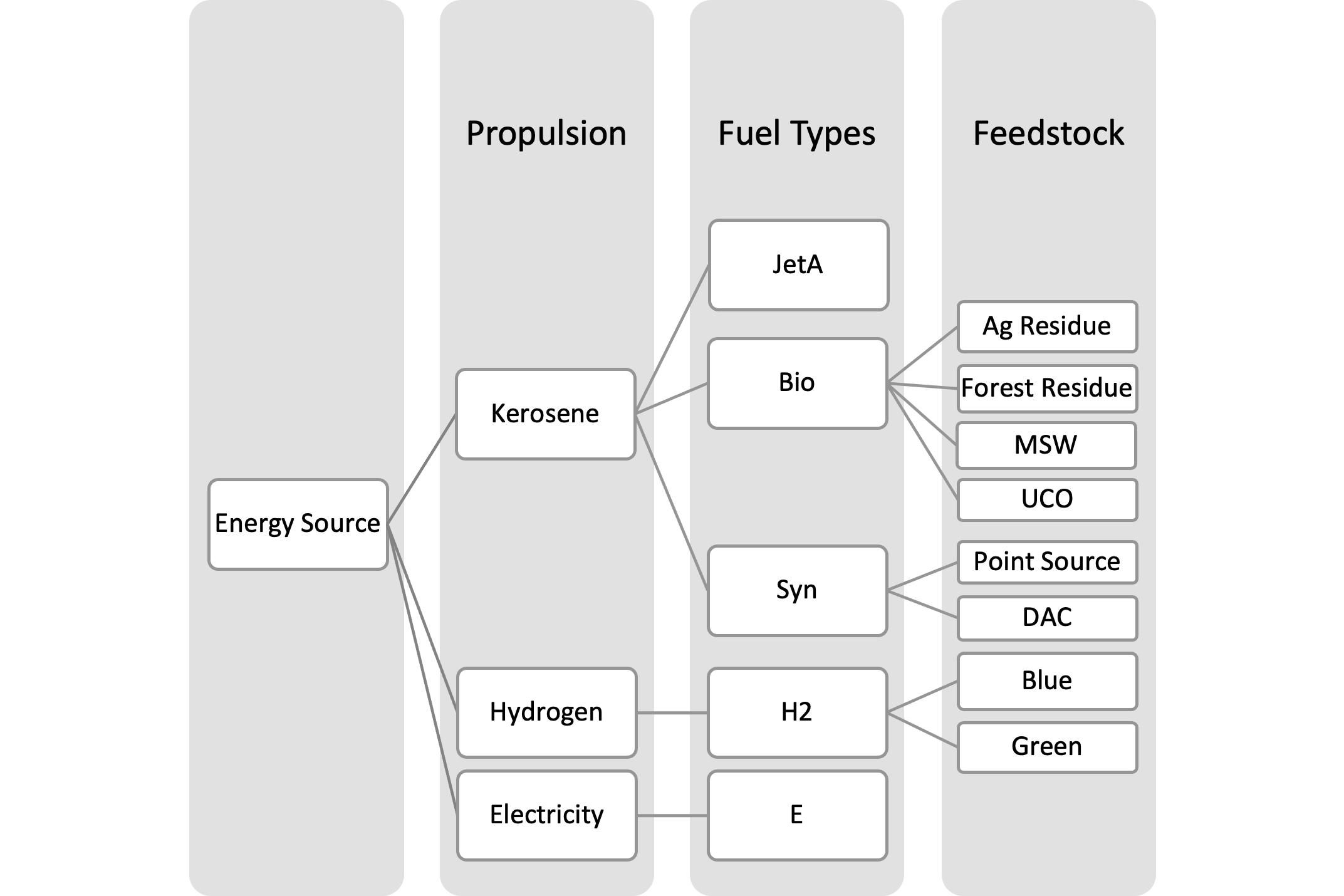
Figure 3. Propulsion methods and fuel types modelled. Fuel type names and feedstock names are specific variable names used in the model.
First, the model calculates the total energy demand for each segment (propulsion specific), for both passenger and freight operations:
\[MJ = RTK*\frac{\text{MJ}}{\text{RTK}} + FTK*\frac{\text{MJ}}{\text{FTK}}\]The model takes user-provided assumptions on SAF supply at the country or regional level and translates them into global averages that can be applied consistently across all aviation segments. First, SAF volumes are aggregated from the country level up to the model’s regional structure. Regional values are then summed into a single global supply pool, under the simplifying assumption that SAF is traded internationally and not restricted to the regions where it is produced.
Once the total global supply is calculated, it is compared against the model’s projection of total kerosene demand. If global SAF supply is less than demand, the remainder is assumed to be met by conventional fossil jet fuel. If SAF supply exceeds kerosene demand, the entire demand is fulfilled by SAF, with the mix of bio-based and synthetic fuels determined by the user-specified feedstock shares.
The model then calculates the weighted average GHG intensity of each fuel type (JetA, Bio, Syn, H2, and E) based on feedstock shares. Since hydrogen and electricity only have one fuel type respectively, their GHG intensity are simply those of “H2” and “E”. The GHG intensity of each segment is then calculated based on the volume split of feedstocks.
6. Emissions
The Emissions Module translates segment-level fuel and energy use into pollutant mass emissions and contrail effective radiative forcing. For each segment s and propulsion type p, the module first computes CO₂ emissions as:
\[E_{CO_{2},s,p} = F_{s,p} * CI_{p}\]where \(F_{s,p}\) is the total fuel consumption (MJ) from the Energy Module, and \(CI_{p}\) is the GHG intensity of the fuel blend \((\frac{gCO_{2}e}{MJ})\) calculated in the Fuels Module.
Short-lived climate pollutants (SLCPs) are estimated by applying emission indices to fuel burn:
\[E_{i,s,p} = F_{s,p} + EI_{i,p}\]where $EI_{i,p}$ (g/kg fuel) represents the emission index of pollutant i (e.g., NOₓ, SOₓ, H₂O, nvPM). Each pollutant stream can then be modified by reduction factors $R_{i,p}$ representing mitigation from engine technology improvements or alternative fuels:
\[E^{adj}_{i,s,p} = E_{i,s,p} * (1 - R_{i,p})\]Specifically, for kerosene propulsion segments, the fractional change in nvPM emission index (both nvPM mass and number) due to SAF blending is modeled as a quadratic function of the SAF blend percentage (0–100%):
\[∆EI_{nvpm}(\%) = 0.0039*(saf\%)^{2} - 0.8171*(saf\%)\]Sulfur is assumed to scale linearly with the fossil fuel fraction:
\[E^{adj}_{SO_{2}} = (1-saf\%) * EI^{JetA}_{SO_{2}}\]Contrail radiative forcing is treated distinctly from direct emissions. It scales with total flight distance $D_{s}$:
\[\text{ERF}_{contrail,s,p} = D_{s} * CF_{p} * (1 + R_{i,p})*(1-A_{s})\] \[D_{S} = RTK_{S} * \text{PayloadEfficiency} * \text{TrafficEfficiency}\]where $CF_{p}$ is the contrail forcing intensity (mW/m² per km), $R_{i,p}$ is the contrail reduction factor (negative value) as a function of nvPM intensity change, and $A_{s}$ is the user-defined contrail avoidance rate for segment s.
To calculate the contrail reduction factor, the fleet-average nvPM number emission index (particles/kg fuel) is computed first:
\[EI^{num}_{nvpm} =\frac{\Sigma_{flights}nvPM_{num}}{\Sigma_{flights}Fuel(kg)}\]When the average nvPM number EI is greater than $10^{13}$ particles per kg (i.e., soot rich regime), the impact on ice particle number (IPN) is scaled linearly with the change in nvPM number EI:
\[∆IPN(\%) = 1.1579 * ∆EI_{nvpm}\]The change in IPN translates to a percentage change in contrail effective radiative forcing (ERF):
\[∆ERF_{contrail}(\%) = 0.6084 * ∆IPN\]Then:
\[ERF^{adj}_{contrail} = ERF^{JetA}_{contrail} * (1 + \frac{∆ERF_{contrail}}{100})\]When the average EI is less than \(10^{13}\) particles per kg (i.e., soot-poor regime), contrail ERF changes are not computed from the quadratic fit above. Instead, they are taken from exogenous delivery-year specific engine contrail reduction factors; this is because, in a soot-poor environment, water vapor and volatile particles from sulfur and lubrication oil become the dominant sources of ice nuclei. The fleet-average engine contrail reduction factors ($R_{engine}$) are applied as below:
\[ERF^{adj}_{contrail} = ERF^{JetA}_{contrail} * R_{engine}\]All pollutant emissions are aggregated by segment and year, producing both fuel-specific totals and global aviation emission inventories. When scenario inputs specify SAF blending or ZEP adoption, the corresponding changes in fuel GHG intensity, engine emission factor, and contrail avoidance rate are applied consistently across the calculation chain.
7. Demand
The Demand Module translates the increase in fuel price to an increase in ticket price, and estimates demand response based on air travel’s demand elasticity to price. Fuel price in each year is estimated from baseline Jet A costs and SAF cost assumptions input by the user. Hydrogen and electricity, which are estimated to be lower cost fuels than SAFs for relevant segments, are not used to estimate demand response.
This analysis leverages the operations details from ICCT’s JETSTREAM model, which includes 82,694 route-aircraft type combos. Route-specific 2019 average economy-class airfare data were purchased from RDC; the data covers almost half of the 2019 passenger operations. For routes not covered by the dataset, we estimated their fare based on extrapolated “dollar per km” by stage length and by region. Demand elasticities are also matched to routes based on ICAO region pair and short vs. long haul. Pan-national level price elasticities are derived from InterVISTAS consultant report to IATA. The more detailed Boeing region pairs used in the model are matched to corresponding ICAO region pairs in advance.
Table 2. Air travel’s demand elasticities to price used in the model.
| Region Pair | Long-haul | Short-haul* |
|---|---|---|
| Africa-Africa | -0.36 | -0.4 |
| Africa-Asia/Pacific | -0.6 | -0.66 |
| Africa-Europe | -0.6 | -0.66 |
| Africa-Latin America/Caribbean | -0.72 | -0.79 |
| Africa-Middle East | -0.6 | -0.66 |
| Africa-North America | -0.72 | -0.79 |
| Asia/Pacific-Asia/Pacific | -0.57 | -0.63 |
| Asia/Pacific-Europe | -0.54 | -0.59 |
| Asia/Pacific-Latin America/Caribbean | -0.36 | -0.4 |
| Asia/Pacific-Middle East | -0.57 | -0.63 |
| Asia/Pacific-North America | -0.36 | -0.4 |
| Europe-Europe | -0.84 | -0.92 |
| Europe-Latin America/Caribbean | -0.72 | -0.79 |
| Europe-Middle East | -0.54 | -0.59 |
| Europe-North America | -0.72 | -0.79 |
| Latin America/Caribbean-Latin America/Caribbean | -0.75 | -0.83 |
| Latin America/Caribbean-Middle East | -0.6 | -0.66 |
| Latin America/Caribbean-North America | -0.6 | -0.66 |
| Middle East-Middle East | -0.57 | -0.63 |
| Middle East-North America | -0.6 | -0.66 |
| North America-North America | -0.6 | -0.66 |
*Short-haul flights are defined as less than 1,500km in great circle distance, and all other flights are categorized as “long-haul” for the purpose of matching elasticities.
In each analysis year, the module updates the total passenger count, fuel burn, and emissions for each route-aircraft type combo, based on the segment-level changes in traffic and energy consumption compared to previous year. The change in demand for each route-aircraft combo is then calculated based on the increase in ticket price, as below:
\[PriceInce = \frac{\text{FuelBurn}\left\lbrack L \right\rbrack}{\text{TotalPax}}*FuelCostDiff\left\lbrack \frac{\$}{L} \right\rbrack*PassThrough\] \[PctPriceInc = \frac{PriceInc + AvgFare}{\text{PriceInc}}\] \[NewPax = TotalPax*\left( 1 + Elasticity*PctPriceInc \right)\] \[NewRPK = NewPax*Distance\]The PassThrough variable refers to the percentage of increase in fuel costs that airlines typically pass on to consumers by increasing ticket prices. This pass-through rate is a user input.
The percentage of RPK change is summarized based on segment and passed on to the next iteration of the model, feeding into the Traffic Module. The updated fuel burn, emissions, and fare are also passed on for the next iteration of the Demand Module.
This module also calculates the implied carbon price from the fuel price increase. Near-term carbon prices were modeled as a fossil fuel levy and cross-subsidy to alternative fuels, while long-term carbon prices equal to the marginal cost of alternative fuels. Specifically, carbon prices are estimated in each year as the lesser of:
-
A cross-subsidy from fossil jet fuel to SAFs ($ of incremental SAF cost/tonnes of total aviation CO2)
-
A classic marginal abatement cost ($ of incremental SAF cost/tonnes of SAF CO2 abatement)
Scenario inputs
The PACE model can take in various user inputs for modeling customized scenarios. The table below shows the user/scenario inputs for ICCT’s Vision 2050 report.
Table 3. Model inputs that offer flexibility through user definition.
| Variables | Definition | Units |
|---|---|---|
| Technical Efficiency | New aircraft fuel efficiency, relative to base year | fraction |
| Payload Efficiency | Share of maximum structural payload carried by airlines; proxy for load factor and one input into operational efficiency, relative to base year | fraction |
| Traffic Efficiency | Relative airport and air traffic management efficiency; one input into operational efficiency, relative to base year | fraction |
| Formation Flying | Formation flying scaler for traffic efficiency | -— |
| Fleetwide Efficiency | Product of base year efficiency and technical, payload, and traffic efficiency | MJ/RPK |
| ZEP Sales Share | Sales share of zero-emission planes | % |
| ZEP Sales Number | Number of zero-emission planes delivered | -— |
| SAF Blend | Country or region average SAF blending ratio | % |
| SAF Cost | SAF price | $/L |
| Feedstock Share | Share within a fuel type based on volume | % |
| Pass Through | Fuel cost increase passed on to consumers | % |
| Modal Shift | RPK shifted to rail by segment | % |
| Engine NOx | Fleetwide engine NOx emission factor and new engine NOx emission factor, relative to base year | fraction |
| Engine PM | Fleetwide engine PM emission factor and new engine PM emission factor, relative to base year | fraction |
| Contrail Avoidance | Share of contrail-producing flights with avoidance maneuvers implemented, by route group | % |
Future work
We are planning to extend the model’s capability for conducting country-level analyses. Our base year data have country details, so the model could either downscale results to countries or take in country-specific inputs to make projections.
The model can also add functionality to model varying utilization rates of aircraft at different ages (by incorporating utilization curves) as well as potential aircraft scrappage policies.
Glossary
Bio: biofuel, fuel derived from biomass
CAGR: compound annual growth rate
CO2: carbon dioxide
Contrails: condensation trails
CY: current year
DAC: direct air capture
DY: delivery year
EJ: exajoule
ERF: effective radiative forcing
FTK: freight tonne kilometers
JETSTREAM: Jet and Turboprop Simulations for Trajectory-based Emissions and Meteorological Effects (ICCT’s aviation inventory model)
GHG: greenhouse gas
IATA: International Air Transport Association
ICAO: International Civil Aviation Organization
ICCT: International Council on Clean Transportation
LH2: liquid hydrogen
MJ: megajoule
MSW: municipal solid waste, as a source of aviation fuel
NOx: nitrogen oxides
p.a.: per annum
PACE: Projection of Aviation Climate Effects model
RPK: revenue passenger kilometers
RTK: Revenue tonne kilometers
SAF: sustainable aviation fuel
SLCP: short-lived climate pollutants
Syn: synthetic fuel, or power-to-liquids fuel
UCO: used cooking oil as a source of aviation fuel
ZEP: zero-emission planes, either hydrogen or electricity powered.