FATE v0.3 Documentation

7/14/2021

Table of contents

• Introduction
  • Sectors
  • Species
• Air quality methods
  • PM_2.5
  • O₃
• Health impact assessment methods
  • Future baseline disease rates

Introduction

The Fast Assessment of Transportation Emissions (FATE) model evaluates air quality and health impacts associated with present or future changes in air pollutant emissions from 9 sectors, including 3 transportation sub-sectors. The tool estimates the national population-weighted ambient PM_2.5 exposure (annual average in µg/m³) for 181 countries and ozone (O₃) exposure (6-month average of the 1hr or 8h daily maximum O₃ in ppb) for 19 individual G20 countries and 24 additional EU member countries. It also outputs the number of premature deaths and disability-adjusted life years (DALYs) associated with exposure to these two pollutants. Supplementary outputs of the tool include baseline exposures to ambient PM_2.5 and O₃ and detailed health impacts by ambient pollutant, disease, and age group. Health outputs of the tool also include 5th and 95th percentile estimates that reflect uncertainty in the concentration-response relationship.

FATE is a reduced-complexity air quality model, allowing users to simulate multiple global scenarios without the high computational costs usually required by chemical transport models. The extent to which exposures of PM_2.5 and O₃ are sensitive to changes in pollutant emissions, denoted as sensitivities, are calculated using the adjoint of the GEOS-Chem model. The health impacts associated with exposure to these pollutants are calculated using methods consistent with the GBD 2019. The tool is designed to accommodate future updates to GBD health impact assessment methods. To estimate health impacts in future years, the tool considers projected changes in population, age distributions, and baseline disease rates.

The main user inputs are absolute or relative changes in emissions (unit: tonnes or %) emitted either at the country scale (in which case the tool applies gridding algorithms) or in user-specified grid cells (choices: GEOS-Chem global 2° × 2.5° grid or 0.1° × 0.1° grid) in specified years (choices: 2019–2050). The tool enables the user to run either a single scenario or a batch including multiple scenarios.

FATE provides the most detail within the transportation sector, however there are no limitations preventing analyses of other supported sectors as well. Supported sectors and emissions are described in the tables below.

Sectors

Abbreviation	Description
WST	Waste
AGR	Agriculture
ENE	Energy
IND	Industry
RES	Residential
SHP	Shipping
TRA_GSL	Road transport gasoline (+ other non-diesel fuels)
TRA_MD	Road transport diesel
TRA_OTH	Other non-road transport (but excluding all shipping)
SHP	Shipping

Species

Abbreviation	Chemical species	Emitted species
BC	Primary black carbon	Carbon (C)
OC	Primary organic carbon	Carbon (C)
NH3	Ammonia	Ammonia (NH3)
NOx	Nitrogen oxides	Nitrogen (N)
SO2	Sulfur dioxide	Sulfur dioxide (SO2)
CO	Carbon monoxide	Carbon monoxide (CO)
VOC	Non-methane volatile organic compounds	≥C4-alkanes, formaldehyde (HCHO), ethane (C2H6), propane (C3H8), propene (C3H6), acetone, methyl ethyl ketone and acetaldehyde (all units are C)

Air quality methods

FATE estimates national population-weighted concentrations of PM_2.5 and O₃ using sensitivities derived from the adjoint of the GEOS-Chem model. The adjoint of the GEOS-Chem model calculates the sensitivity of a population-weighted pollutant exposure (PM_2.5 or O₃) to an emissions perturbation in any of the global model’s 2° × 2.5° grid cells. These sensitivities are output from the GEOS-Chem adjoint as gridded coefficients, which can then be multiplied by emission perturbations to estimate changes in exposure. Note that since the adjoint calculation is a local linear approximation of the sensitivity around the emissions magnitude used in GEOS-Chem, there is some uncertainty in modeling large emission perturbations.

The adjoint sensitivities are calculated for chemical species, thus they do not vary by sector. The coefficients are provided as 2D arrays for surface-layer emissions; this impacts use of these sensitivities for e.g. aviation and electricity generation sectors, where the altitude of the emissions would cause the pollutant response to be different than the same mass of emitted species from a sector emitting only at the surface.

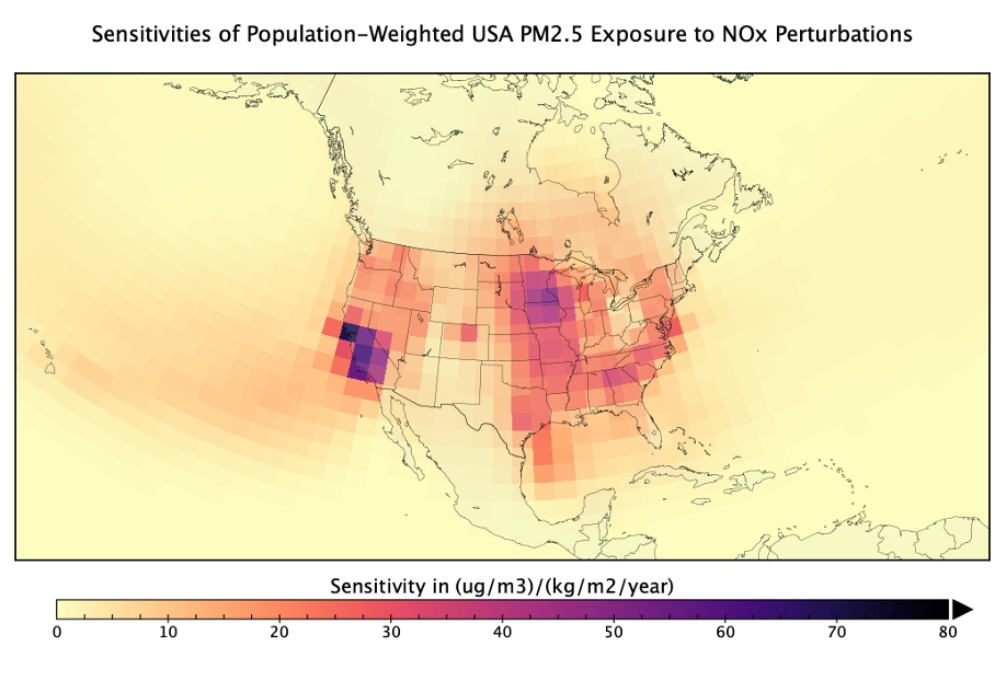
Figure 1. Subset of USA population-weighted PM_2.5 adjoint sensitivities for NOx emissions

PM_2.5

The adjoint response coefficients for the PM_2.5 calculations give the sensitivity of population-weighted annual average PM_2.5 to emissions of BC, OC, NH3, NOX, and SO2. FATE supports 165 countries; an example of the sensitivity of USA PM_2.5 exposure to NOx emissions is shown in Figure 1.

Figure 2. Countries with PM_2.5 sensitivities

The national population-weighted PM_2.5 annual average concentrations (i.e., exposures) are calculated using satellite-derived estimates of surface PM_2.5 concentrations at the 0.1º × 0.1º scale applied as downscaling factors to the GEOS-Chem model’s PM_2.5 concentrations at the 2° × 2.5° resolution. The GEOS-Chem adjoint is then run at the 2° × 2.5° resolution to calculate the emission response coefficients. Using the fine-scale concentrations of the satellite-derived products improves the estimation of population exposure without changing the overall modeled value of PM_2.5 concentrations at the coarse scale. However, given that there are appreciable differences between GEOS-Chem simulated PM_2.5 concentrations and those of the satellite-based product at the coarse scale, we also include an option to adjust (“rescale”) the PM_2.5 concentrations to match those from the satellite-based product, as the latter has been calibrated against a large collection of available in-situ measurements for 2010. For some applications using the adjoint sensitivities to estimate concentrations for years far from 2010, it may be desired to adjust the calculations to remove the rescaling because the satellite-derived estimates would no longer be representative of pollutant exposures.

The adjoint sensitivities can be optionally scaled such that the PM_2.5 health impacts are consistent with the most up-to-date health impact assessment at this time – the GBD 2019 study. With this scaling, FATE is set up such that running the model with ECLIPSE 2019 anthropogenic emissions (the default) results in exactly the country-specific PM_2.5 exposures from the GBD 2019 study.

The adjoint values are computed at the coarse scale, but the user may wish to provide emission perturbations at the fine scale. Within the script we provide a simple mapping of the adjoint sensitivities from the coarse to fine scale.

O₃

For O₃, we directly use simulated surface O₃ concentrations at the 2º × 2.5º resolution. Within the GEOS-Chem adjoint model, the exposures are computed as the maximum 6-month mean of the daily 1-hour maximum O₃. Due to the non-linearity of O₃ chemistry, the local linear response calculated by the adjoint will not be representative of actual changes in O₃ exposure over large changes in emissions. To account for this, we include the option to scale adjoint sensitivities to anthropogenic exposures, calculated from GEOS-Chem, based on input anthropogenic emissions. This methodology is identical to what is done for PM_2.5.

Figure 3. Countries with O₃ sensitivities

The unscaled adjoint sensitivities are the local linear response of a pollutant exposure to changes in emissions and are most applicable over small emission perturbations where the non-linear effects are smaller. The anthropogenic scaled sensitivities are most applicable over larger changes in emissions. We suggest that, if possible, users run scenarios using both the unscaled and scaled sensitivities. Following this, users can choose the more appropriate run and use the difference between the two runs as an uncertainty bound, on either side, to assess uncertainty in the exposure estimate. Rather than propagating this uncertainty into the health calculation, we suggest that users consider uncertainty from the exposure calculation as separate from the health calculation.

O₃ exposure is sensitive to volatile organic compounds (VOCs); however, there are only a few species of VOCs that are considered in GEOS-Chem. For more accurate VOC scenarios, we suggest that users only consider emissions of the following species: ≥C4-alkanes, formaldehyde (HCHO), ethane (C2H6), propane (C3H8), propene (C3H6), acetone, methyl ethyl ketone and acetaldehyde.

The O₃ exposures calculated in GEOS-Chem differ from those used in the GBD 2019 study; the latter incorporate both in-situ monitor observations and simulated concentrations from multiple models using a kriging methodology¹. Consistent with the sensitivities for PM_2.5, an additional scaling factor has been calculated to convert sensitivities from being with respect to the GEOS-Chem exposures (based on the maximum 6-month mean of the 1-hour daily maximum) to being with respect to the GBD 2019 study exposures (based on the 6-month mean of the 8-hour daily maximum).

Health impacts for O₃ can also be assessed using different exposure estimate methods if desired. The O₃ exposure sensitivities are calculated for a metric of the maximum 6-month mean of the daily 1-hour maximum O₃ at the surface level (~50 meters), which is the approximate center altitude of the first layer of GEOS-Chem. Additionally, the maximum 6-month mean O₃ has been calculated for the 8-hour daily max, and adjusted to a height of 2 meters (a level more consistent with O₃ exposure), and the ratio of these two quantities are provided as scaling factors for each country. These ratios can be applied by the user (to the total exposure, adjoint coefficients, and natural exposure in each country) to estimate health impacts based on the maximum 6-month mean of daily 8-hour max concentrations at the 2m height, rather than the 6-month mean of daily 1-hour max at ~50 m.

Health impact assessment methods

The health impacts of PM_2.5 and O₃ exposure are calculated for each country using the “attributable fraction” approach. This approach is widely used by the GBD study², the World Health Organization³, the U.S. Environmental Protection Agency⁴, and throughout the peer-reviewed literature. For each scenario, FATE estimates the number of cases of various health endpoints by age group attributable to each pollutant.

Health impact methods are consistent with the GBD 2019 study, published in June 2020. GBD studies are broadly respected and increasingly used to inform public health decision-making around the world, at all geopolitical levels – international, national, and sub-national. Risk-outcome pairs are only included in the GBD after thorough review of the epidemiological, toxicology, and human and animal study evidence. The GBD is published annually and is updated over time to reflect the evolution of the state of the science, including in epidemiology and air pollution exposure science.

Consistent with the risk-outcome pairs in the GBD, FATE calculates cases of the following health outcomes associated with PM_2.5:

• stroke

• ischemic heart disease

• chronic obstructive pulmonary disease (COPD)

• lower respiratory infection

• lung cancer

• diabetes mellitus type 2

For O₃, only cases of COPD are considered.

The equation used to calculate the disease burden associated with PM_2.5 and O₃ concentrations is:

\[M_{a,i,h} = \text{Pop}_{i} \times \ \text{Popfrac}_{a,h} \times Y_{a,c,h} \times \left\lbrack \frac{\text{RR}_{a,i,h} - 1}{\text{RR}_{a,i,h}} \right\rbrack\]

Where:

• \(M\) is the disease burden (pollutant-attributable deaths or years of life lost) in geographic unit \(i\) for age group \(a\) and health endpoint \(h\)

• \(\text{Pop}\) is the population in the geographic unit \(i\)

• \(\text{Popfrac}\) is the population fraction for age group \(a\) and health endpoint \(h\)

• \(Y\) is the baseline incidence rate (deaths or years of life lost per 100,000 people) in country \(c\) for age group \(a\) and health endpoint \(h\)

• \(\text{RR}\) is relative risk in grid cell \(i\) for age group \(a\) and health endpoint \(h\)

The quantity in brackets is the population attributable fraction – the fraction of disease in a population that is attributable to the risk factor (in this case annual average PM_2.5 or six-month average of 8-hour daily maximum O₃).

A key feature of the PM_2.5 concentration-response curves is that they are nonlinear and flatten considerably at high concentrations, particularly for cardiovascular health endpoints. The shape of the concentration-response curve implies that sensitivity of health effects to a unit change in PM_2.5 concentration in very polluted environments is diminished compared to that in clean environments. Therefore, rather than using a continuous parametric function, we use RR lookup tables, which are provided by the GBD 2019. RRs between concentration points in the lookup tables are linearly interpolated.

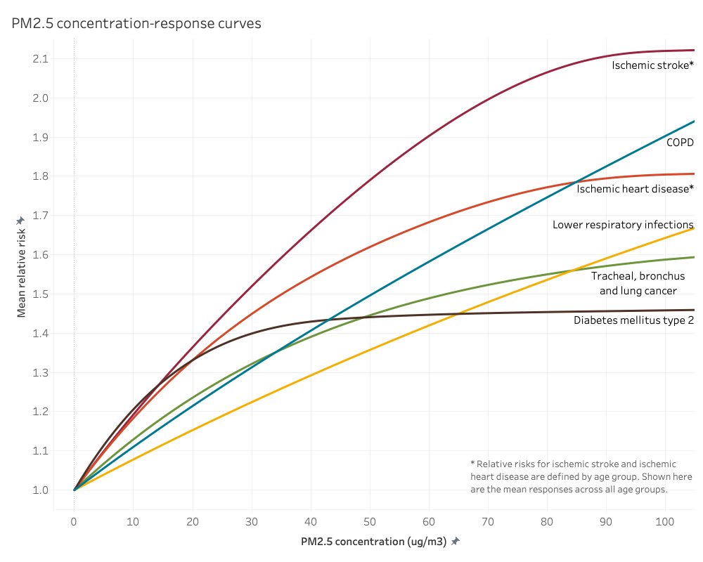
Figure 4. PM_2.5 concentration-response curves for each health endpoint. Ischemic stroke and heart disease have different curves for each age group, however just the mean response is shown here.

For O₃, the same RR estimate is used at all concentrations: 1.06 (95% CI 1.03, 1.10) per 10 ppb O₃ increase (six-month average of the 8-hour daily maximum). This RR is based on five studies of long-term O₃ exposure and COPD from Canada, the United Kingdom, and the United States. We assume the concentration-response curve for O₃ is log-linear (the natural log of RR is linearly associated with O₃ concentration). With this assumption, a RR of 1.06 translates to a concentration-response factor of 0.005827 (calculated by \(\ln{(\frac{\text{RR}}{10})}\)). This assumption is also used by the GBD⁵ and throughout the scientific literature.

The GBD 2019 study calculates the health burden from O₃ exposure above a theoretical minimum risk exposure level (TMREL) taken from a uniform distribution between 29.1 – 35.7 ppb. We cut off any calculation of risk below the midpoint of this range, 32.4 ppb. We have decided not to use a TMREL for PM_2.5 as use of the model typically focuses on smaller perturbations in concentrations well above the TMREL. In addition, epidemiological studies are finding PM_2.5 mortality effects at lower and lower concentrations, down to approximately 2 µg/m³, so calculating health impacts at very low concentrations is justified by the current evidence. The TMREL is more important for O₃, however, because it’s a larger fraction of the total concentration.

Future baseline disease rates

GBD 2019 gives annual baseline disease rates up to 2019, however a key feature of FATE is estimating the impacts of exposure changes into the future. In order to determine a baseline for projected disease rates we refer to the GBD Foresight project⁶. We use their values through 2040, extending the 2040 rates forward for any years beyond. The dataset of future disease rates for each of the causes affected by air pollution was created by Rita Van Dingenen from Joint Research Centre of the European Commission. As the GBD Foresight projections were based on the GBD 2015 study, Van Dingenen scaled the original GBD Foresight future rates by the ratio of GBD 2017 to GBD 2015 values for the year 2015. Rates for diabetes mellitus type 2 are held constant at present-day levels since the Foresight project only provided future rates for type 1 and type 2 diabetes together.

Scaling was performed for each cause, land, age group:

\[\text{GBDForesight}_{\text{Scaled}(\text{Year})} = \text{GBDForesight}_{\text{Download}(\text{Year})} \times \ \frac{ {\text{GBD}2017}_{2015}}{\text{GBDForesight}_{\text{Download}(2015)}}\]

We then performed further rescaling to be consistent with the GBD 2019 to avoid a substantial disconnect between historical and projected baseline rates. To rescale to the 2019 values, we first calculated the annualized percent change in Van Dingenen’s estimates from 2015-2020, 2020-2025, and so on until 2040. Then we matched these to the corresponding country-cause-age combination in the GBD 2019 data for 2019. We applied the 2015-2020 annualized rate for one year to calculate 2020 projected values from the 2019 data, then we applied the other rates to calculate annual projections to 2040.