AZTEC v1.1 Documentation
AZTEC User Guide
The Analyzer of Zero-emission Transportation Energy and Costs (AZTEC) model is an upgraded version of the ICCT’s first fleet-level total cost of ownership (TCO) tool, the Toolkit for Urban Bus Operations (TURBO).
Table of Contents
- Introduction
- Model Inputs
- Run Settings
- Modules
- Model outputs
- Sensitivity analysis
- Appendix
Introduction
The AZTEC model supports the technical analysis of vehicle fleets in two key areas:
1. Fleet level emissions modeling
- Annual air pollutant and GHG emissions by vehicle type, powertrain technology, and fuel type for user defined procurement pathways
- Evaluate scale and pace of emissions changes resulting from fleet technology transitions
- Route level energy demand modeling
- Example application: Evaluation of São Paulo Climate Change Law
2. Fleet level TCO assessment
- Comparative assessment of the TCO of conventional and alternative fleet technologies and fuels
- Example application: TCO assessments for São Paulo and Johannesburg
Acknowledgments
AZTEC was first developed in 2022 by Gabe Hillman Alvarez, Erik Pronk, Josh Miller, and Arijit Sen. Version 1.1 was developed in 2024 by Gabe Hillman Alvarez, Jakob Schmidt, Hussein Basma, and Arijit Sen.
Model Inputs
Inputs to AZTEC are defined in the configuration file. These inputs define how the model should be run, including what data to use, which modules to include, and basic run settings.
This section outlines what inputs are required, what detail they should have, and what are the default options.
Overview
AZTEC comes with a few default inputs, but most of the required data sets are specific to the region of analysis. Each input data set is expected to follow a common format and be saved as a .csv file. All inputs should be self-descriptive, and to help enforce this they are required to have a Variable or Parameter column, as well as a Unit column. Below are a couple examples of data inputs.
General Structure
Data inputs will contain a subset of these standard columns:
| Column | Example Values | Description |
|---|---|---|
| Scenario | “Baseline”, “Scen 1” | The name of the scenario. |
| Region | “IND”, “Bangalore” | The region of analysis. |
| Route | “Route 1”, “51A” | Used to distinguish between multiple routes within a single region. |
| Vehicle | “Single Bus 12 M”, “Articulated” | The types of vehicles in your current or projected fleet. Vehicle names can be arbitrary, but must remain consistent across all inputs. |
| Technology | “diesel”, “EV”, “hybrid”, “CNG” | The engine powertrain technology. Any value is accepted, but default PM2.5 speciation profiles are only provided for gasoline, diesel, biodiesel, ethanol, and CNG vehicles. |
| Control | “Euro V”, “BEV”, “EV_324kWh” | The emissions control technology used by the engine. Any value is accepted, but default PM2.5 speciation profiles are only provided for “Euro 0” through “Euro VI”. |
| Fuel | “B20”, “CNG”, “electricity”, “diesel” | Specific fuel type used by the vehicle. Fuels must match values in fuel_shares and ghg_emission_rates inputs. |
| Component | “Battery”, “Other Components” | Constituent part of vehicle. May be purchased, financed, and sold independently of vehicle. |
| Replacement | “0”, “1”, “2” | 0 for original component, 1 for first replacement, 2 for second replacement, etc. |
| InfrastructureType | “Fast Charging Station”, “Fuel Station” | Infrastructure used to deliver energy to vehicle fleet. |
| CostTier | “Tier 1”, “Tier 2” | Different tiers for energy costs, to capture, e.g., different energy prices at different times of day. |
Two important points about the data requirements:
- Units are automatically checked before running. Required units are shown in the tables below.
- Two different years are used in AZTEC: calendar year (CY), i.e., the year the action, cost, or payment occurs; and model year (MY), i.e. the year the object entered the fleet. To eliminate the possibility of confusion, only CY data should be pivoted wide (i.e. provided as additional columns).
Example Activity Input
The Region column is required for most variables. Average annual vehicle activity per vehicle (km/yr/vehicle) can be specified for the whole fleet by leaving out the Vehicle column.
Note: The ellipsis ‘…’ in the following table indicates that columns could be added for additional years; however, ‘…’ is not a valid column name or value.
| Region | Variable | Unit | Vehicle | 2018 | 2019 | … | 2038 |
|---|---|---|---|---|---|---|---|
| Bangalore | Activity | km/yr/vehicle | Midi | 70000 | 70000 | … | 70000 |
| Bangalore | Activity | km/yr/vehicle | Standard | 70000 | 70000 | … | 70000 |
Example Service Lifetime Input
Some variables are not temporal. In this case, the column containing the values should be called Value.
| Region | Variable | Unit | Vehicle | Value |
|---|---|---|---|---|
| Bangalore | Vehicle service lifetime | Year | Midi | 12 |
| Bangalore | Vehicle service lifetime | Year | Standard | 12 |
More examples can be found in AZTEC’s example/inputs/ directory.
Interpolation
For many inputs, AZTEC interpolates between missing years, allowing for smaller and clearer input tables. Missing values are generally filled in with a basic linear interpolation. While there cannot be missing values for the base year, missing future years are forward filled from the last existing value.
As an example, consider a scenario where projected sales for standard type buses switch from Euro V to Euro VI in 2023, then steadily switch to BEB until 2028.
This input could look as follows:
| Region | Variable | Unit | Vehicle | Technology | Control | 2020 | 2022 | 2023 | 2028 |
|---|---|---|---|---|---|---|---|---|---|
| São Paulo | Sales | vehicle | standard | diesel | Euro V | 500 | 500 | 0 | |
| São Paulo | Sales | vehicle | standard | diesel | Euro VI | 0 | 0 | 500 | 0 |
| São Paulo | Sales | vehicle | standard | electricity | BEB | 0 | 0 | 500 |
The above table is interpreted by AZTEC identically to the following table:
| Region | Variable | Unit | Vehicle | Technology | Control | 2020 | 2021 | 2022 | 2023 | 2024 | 2025 | 2026 | 2027 | 2028 |
|---|---|---|---|---|---|---|---|---|---|---|---|---|---|---|
| São Paulo | Sales | vehicle | standard | diesel | Euro V | 500 | 500 | 500 | 0 | 0 | 0 | 0 | 0 | 0 |
| São Paulo | Sales | vehicle | standard | diesel | Euro VI | 0 | 0 | 0 | 500 | 400 | 300 | 200 | 100 | 0 |
| São Paulo | Sales | vehicle | standard | electricity | BEB | 0 | 0 | 0 | 0 | 100 | 200 | 300 | 400 | 500 |
These input files will not be interpolated. So, users must specify them for all years and ages, where relevant.
- Stock
- Transmission loss
- ISO map
- PM profiles
- Projections
- Survival curves
- Infrastructure base year stock
- Vehicle service lifetime
- Stakeholders
These input files will have missing calendar years filled in with a linear interpolation where possible. Additionally, the last provided value will be forward filled to all future years.
- Sales
- Activity
- Energy intensity
- Fuel shares
- Grid mix
- Emission factors
- GHG emission rates
- GHG electric generation
- Infrastructure annual costs
- Vehicle-level costs
- Energy costs
- Energy usage share
- Revenue
- Taxes and subsidies
These input files are specially interpolated.
- Infrastructure purchases: Forward filled by calendar year, including for missing intermediate years.
- (Vehicle/component and Infrastructure) financing and costs: “Cost”, “Incentive”, and “Down payment” are linearly interpolated by model year (MY), and all other parameters are forward filled. For the vehicle/component financing and costs, “Useful lifetime” is also backfilled to the earliest MY present in the base-year stock, so that we have information about when those components will need replacing.
- (Vehicle/component and Infrastructure) age-specific costs: Linearly by calendar year AND age.
- (Vehicle/component and Infrastructure) depreciation: Linearly by age.
Default inputs
The variables below provide default values that are used in the emissions calculations unless specific inputs are provided by the user. To overwrite or add to the default inputs, just include the custom values as an input in the configuration file. For example, GHG emission intensities for a specific fuel can be added/overwritten by including the input ghg_emission_rates = my_fuel_ghg_efs.csv in the configuration file.
Note that although the default versions of ghg_emission_rates and ghg_electric_generation are not annual (i.e., they do not vary across years),
user inputs that override these defaults may optionally have a “CY” column or specify the years wide.
See Energy units for more information about what units are supported if you wish to overwrite these defaults.
| Variable Name | Units | Columns | Description |
|---|---|---|---|
ghg_emission_rates |
g/mmBTU | Region, Fuel, [years] | WTT, TTW, and WTW emission factors of CO2, CH4, and N2O. Defaults for 18 fuels are taken from AFLEET. |
ghg_electric_generation |
g/mmBTU | Region, Electricity_source, [years] | WTW emission rates of CO2, CH4, and N2O per unit of electricity generation by source (power plant type), before transmission and distribution losses are considered. |
transmission_loss |
g/mmBTU | Region, [year] | Electricity transmission and distribution losses (see Transmission Loss). |
pm_profiles |
share | Technology, Control, Value | PM2.5 speciation profiles for BC and OC (see PM2.5). |
Required inputs
AZTEC’s three modules – Fleet Turnover, Emissions, and Total Cost of Ownership (TCO) – are not independent. Emissions requires Fleet Turnover to be run, and TCO requires that both Fleet Turnover and Emissions be run. The Module column in the table below specifies for which module(s) the following inputs are required.
Note: All inputs are required to have the columns Variable and Unit. Region and Route are optional where Vehicle is allowed.
| Variable Name | Units | Columns | Module | Description |
|---|---|---|---|---|
stock |
vehicle | Vehicle, Technology, Control, Age, [baseline year] | Fleet Turnover, Emissions | Number of vehicles in the base year fleet. |
activity |
km/yr/vehicle | Vehicle (optional), [years] | Emissions, TCO | Average annual vehicle activity per vehicle for each year. If Vehicle column is not given, the inputs provided are applied to all vehicle types. |
sales |
vehicle, share | Vehicle, Technology, Control, [years] | Fleet Turnover | Number of vehicles sold by year or share of vehicles sold within each vehicle type. |
energy_intensity |
See Energy units | Vehicle, Technology, Control, [baseline year] | Emissions, TCO | Energy intensity by vehicle type, technology, and control level. |
emission_factors |
g/km | Vehicle, Technology, Control, [years] | Emissions, TCO | Air pollutant emission factors. |
fuel_shares |
share | Technology, Fuel, [years] | Fleet Turnover, Emissions | Share of each fuel consumed by a given vehicle technology. |
service_lifetime |
year | Vehicle (optional), Value | All | Fixed-length lifetime of the vehicle (may differ from lifetimes of components within the vehicle). Required if turnover_method is “service_lifetime” (see Fleet Turnover), or if TCO is enabled. |
all TCO inputs except stakeholders |
mixed | mixed | TCO | TCO inputs. See TCO. |
Optional inputs
| Variable Name | Units | Columns | Description |
|---|---|---|---|
grid_mix |
share | Region, Electricity_source | Share of electricity generation by power plant type. This is required for scenarios where electricity is a fuel. If local grid distribution data is not available, country-level generation mixes can be sourced from the IEA (see GHG Emissions). |
iso_map |
unitless | Region, ISO | Map of modeled regions to standard ISO codes, to look up default transmission loss data. Required if grid mix provided. |
projections |
vehicle | Vehicle (optional), [years] | Projected total stock. Required if growth_method is “projected” (see Fleet Turnover). |
survival_curves |
unitless | tm, km | Parameters for survival curves. Required if turnover_method is “survival_curve” (see Survival Curves). |
stakeholders |
unitless | Vehicle (optional), FinanceModule, CostStakeholder, RevenueStakeholder | Assigns different stakeholders (e.g., Transit Authority) to different cash flows (see Stakeholders). |
Energy units
All inputs which concern quantities related to energy (e.g, energy intensity, emissions factors, energy costs) support automatic unit conversion to MJ from the following units:
- kWh
- DLE
- GLE
- mmBTU
- m3 (for natural gas)
- kg (for hydrogen)
All energy-related outputs report in MJ.
Run Settings
These inputs define the scope of the analysis and must be specified in the Settings section of the configuration file.
| Variable Name | Description |
|---|---|
data_dir |
Path to the directory where the inputs will be read from. |
output_dir |
Path to the directory where the outputs will be written. |
base_year |
The base year for which stock data are provided. All required temporal inputs should have this year as a column. |
end_year |
The last year of analysis (inclusive). |
growth_method |
Fleet growth method for fleet turnover calculations. One of constant, projected or None. |
purchase_method |
Method for purchasing new vehicles for fleet turnover calculations. One of scheduled or None. |
turnover_method |
Method for retiring vehicles for fleet turnover calculations. One of service_lifetime, survival_curves or None. |
use_emissions |
Run the Emissions module? True or False. |
use_tco |
Run the Total Cost of Ownership module? True or False. |
use_stakeholders |
Are you supplying a cost/revenue stakeholder map? True or False. |
export_detailed_tco |
Would you like to report detailed costs (broken down by MY/Age in addition to CY)? True or False. |
Modules
Fleet Turnover
One of the core features of AZTEC is projecting fleet turnover. The vehicle fleet at a given year is a function of three inputs:
- Purchases - how many new vehicles are sold
- Growth - how much the total fleet grows
- Retirements - how many vehicles are retired from the fleet
Any of these three factors can be calculated from the other two. AZTEC supports the following:
| Configuration | Required Inputs | Description |
|---|---|---|
growth_method = projected, purchase_method = scheduled |
<ul><li>sales</li><li>projections</ul> |
This configuration is modeling a scheduled vehicle procurement plan. The sales input gives the number of vehicles purchased by year. Oldest vehicles are retired first, such that Retirements = Purchases - Growth, where fleet growth is the number of vehicles specified by projections. |
growth_method = constant, purchase_method = scheduled |
<ul><li>sales</li></ul> |
This configuration is the same as above, but keeping the fleet size constant rather than projecting growth. Since growth is constant, Retirements = Purchases. |
growth_method = projected, turnover_method = service_lifetime |
<ul><li>sales (shares)</li><li>projections</li><li>service_lifetime</li></ul> |
For this configuration, sales is the share of purchases by technology type and does not determine total sales. To calculate absolute sales, first retirements are determined from the service lifetime and the age distribution of the fleet. Then, purchases are calculated as Purchases = Retirements + Growth. |
growth_method = constant, turnover_method = service_lifetime |
<ul><li>sales (shares)</li><li>service_lifetime</li></ul> |
This configuration is the same as above, but keeping the fleet size constant rather than projecting growth. Retirements are calculated in the same way, then Purchases = Retirements. |
growth_method = projected, turnover_method = survival_curves |
<ul><li>sales (shares)</li><li>projections</li><li>survival_curves</li></ul> |
Turnover is calculated similarly to using the service_lifetime turnover method, but using a survival curve function to retire vehicles. |
growth_method = constant, turnover_method = survival_curves |
<ul><li>sales (shares)</li><li>projections</li></ul> |
This configuration is the same as above, but keeping the fleet size constant rather than projecting growth. |
Fleet Growth
To model a projected change in either the number of vehicles of a specific type or the total number in the fleet, make sure that both growth_method is set to projected and that the input projections is given. The projections input should point to a file containing number of vehicles by vehicle type (optional) and year (required). Any number of years can be given; intermediate years are linearly interpolated.
If you want to model compound growth of the fleet in years between projection targets, please see the devtools folder for a script to help calculate the intermediate targets off-model.
Survival Curves
Retiring vehicles using survival curves is best suited for modeling the natural retirement of vehicles. This is more applicable for private vehicles than public bus fleets, and is generally DISCOURAGED.
The survival curve used in AZTEC is based on the survival function of a Weibull distribution. There are two distribution parameters that we use to define the curves:
- Tm: The scale parameter of the Weibull distribution
- Km: The shape (steepness) parameter of the Weibull distribution
For more details on this methodology see Hao et al., 2011.
Emissions
GHG Emissions
Greenhouse gas emissions are calculated for each year with the formula:
emissions = stock * activity * energy intensity * emission factor
Emission factors for greenhouse gases are fuel specific and take into account fuel lifecycle (WTW) emissions, whereas emission factors for other air pollutants are distance/technology specific and cover only TTW emissions. Default values for many fuels are provided by the AFLEET model and include both WTT and TTW emissions.
To use the AFLEET defaults, all fuels specified in the fuel_shares input must match one of the following:
- canola-based BD100
- canola-based RDII 100
- diesel
- corn oil-based BD100
- palm FFB-based RDII 100
- soybean-based BD100
- soybean-based RDII 100
- tallow-based BD100
- CNG
- CNG shale
- H2 central plants
- H2 refueling electrolysis
- H2 refueling natural gas
- gasoline
- LNG animal waste
- LNG wastewater
- LNG LFG
- LNG conventional
Note: Land-use change emissions are not included in the AFLEET defaults.
GHG emissions from electricity production are also sourced from the AFLEET model. The emissions, in g/mmBTU, are given for 5 power plant types (oil, natural gas, coal, biomass, nuclear) and “other”, which can be used for renewable sources. The user-defined input grid_mix defines the share of generation by power plant type. These values can be found on the IEA’s public Data and statistics website (Data browser –> Topic: Energy supply, Indicator: Electricity generation by source).
Transmission and Distribution Losses
The default values for electricity transmission and distribution losses are from the IEA’s public Data and statistics website. Currently default values are provided most countries and a few larger regions, but users will need to update the default file for smaller regions such as cities if they have higher resolution data. To use the default country-level data, users must map their custom regions to standard ISO codes with the iso_map input. Transmission and distribution losses are calculated as electricity losses (Losses) divided by total electricity production (Total production).
Other Air Pollutants
Air pollutant emissions are calculated for each year with the formula:
emissions = stock * activity * emission factor
The stock data for all years following the base year are the results of the fleet turnover calculations. Activity data are required inputs, and are either linearly interpolated between multiple input years or assumed to remain constant after the base year.
Unless specific emission factors are provided, BC and OC are calculated from PM2.5 emissions.
PM2.5 Speciation
Unless BC and OC emission factors are specified by the user, they are calculated from PM2.5 using speciation profiles. Default speciation profiles are from US EPA’s MOVES2014 model (EPA 2014, MOVES2014 speciation, Table C-1), however alternative values can be given with the pm_profiles input. Speciation is only done if either BC or OC is missing from the emission factor inputs; if just one is provided, it is not used. Default PM2.5 speciation is done for the following vehicle technologies and control levels:
- Vehicle technologies: gasoline, diesel, biodiesel, ethanol, CNG
- Control levels: Euro 0, Euro I, Euro II, Euro III, Euro IV, Euro V, Euro VI
Total Cost of Ownership
The total cost of ownership (TCO) module calculates the costs of vehicle acquisition, maintenance, and operation for each bus type in the fleet. To enable this module, set the input use_tco equal to True.
For the TCO calculations, AZTEC relies on activity, energy intensity, fleet, and emissions information from the earlier two modules. The other TCO inputs must be specified separately in the following files. All TCO inputs are required and must be specified for every vehicle type.
In general, all costs should be provided in real, not nominal, terms. If it is strictly necessary for your project to use nominal inputs, please make sure you have applied your inflation rate consistently to all inputs, and provide the discount rate in nominal terms as well.
Vehicle/Component
Vehicles may be specified by their individual components (e.g., chassis, battery, motor, etc.) or for the whole vehicle. The following inputs contain information about costs and parameters of and related to vehicles or vehicle components.
Note that replacement components are not able to change operational parameters about the vehicle, e.g., energy efficiency or emissions intensity. For help modeling retrofits that you expect to alter vehicle performance, please see the retrofits section.
Vehicle/component financing and costs
- Contents: The anticipated costs and financing structure and details for a specific component (or the full vehicle).
- Please Exclude: Monthly payments, this input is specifically for annualized or lump sum elements
- Example:
example/inputs/tco/vehicle_component_costs.csv - Valid columns: Scenario, Region, Route, Vehicle, Technology, Control, Component, Replacement, MY, Parameter, Unit, Value
- Interpolation: For these, “Cost”, “Incentive”, and “Down payment” are linearly interpolated by MY, and all other parameters are forward filled. For the vehicle/component financing and costs, “Useful lifetime” is also backfilled to the earliest MY present in the base-year stock, so that we have information about when those components will need replacing.
- Parameters included in file:
| Parameter | Allowable Units | Description |
|---|---|---|
| Useful lifetime | Years | Expected length of time a particular vehicle component will be in use. If component useful lifetime exceeds remaining vehicle service lifetime, the component will be sold when the vehicle retires. |
| Cost | Currency ($) | Expected total component cost. The sticker price of the component |
| Incentive | Currency ($) | Any incentives (rebates, discounts) that will be applied to the purchase price directly |
| Down payment | Currency ($) | Upfront payment applied to the principal |
| Finance model | Type | Method for payment of the remaining principal (cost less incentive less down payment): Loan, Lease, or Cash |
| Interest rate | Percentage | (Loans only) Annually accruing interest rate |
| Number of years | Years | (Leases and loans only) Length of the lease or loan term |
| Number of grace years | Years | (Loans only) Years in which payments (on principal, interest or both) are temporarily suspended. Should be zero if Grace type = 0, and should be a positive integer if Grace type = 1 or 2 |
| Grace type | Type | (Loans only) 0 – no grace period 1 – grace period for interest only 2 – grace period for interest and principal |
| Payment per period | Currency ($) | (Leases only) Annual lease payment amount |
For any vehicles or components still in the fleet at the end of the analysis period, any outstanding loan balances will be paid off and they will be sold at their depreciated value. For clarity, the resulting cash flows will be reported in the following year.
Vehicle/component costs, age-specific
- Contents: Any costs for vehicles/components that depend on age
- Please Exclude: age-independent costs, which may be specified in vehicle-level costs
- Example:
example/inputs/tco/vehicle_component_costs_age_specific.csv - Valid columns: Scenario, Region, Route, Vehicle, Technology, Control, Component, Replacement, Age, CY (wide or long), Parameter, Unit, Value
- Interpolation: Linearly, by calendar year and age
- Parameters included in file:
| Parameter | Allowable Units | Description |
|---|---|---|
| Age-specific variable cost | $/km | Variable (activity-dependent) costs that vary with age |
| Age-specific fixed cost | $/vehicle | Fixed (activity-independent) costs that vary with age |
Vehicle/component depreciation
- Contents: The expected depreciation schedule of a vehicle or component
- Please Exclude:
- Example:
example/inputs/tco/vehicle_component_depreciation.csv - Valid columns: Scenario, Region, Route, Vehicle, Technology, Control, Component, Replacement, Age, Parameter, Unit, Value
- Interpolation: Linearly by age
- Parameters included in file:
| Parameter | Allowable Units | Description |
|---|---|---|
| Depreciation | Percentage (%) | Annual depreciation, always referenced to the original cost |
Note that the values here are interpreted as the percent of the original cost that is lost in value each year, NOT the cumulative loss of value up to that point.
E.g., the following input:
| Age | Parameter | Unit | Value |
|---|---|---|---|
| 0 | Depreciation | % | 0 |
| 1 | Depreciation | % | 20 |
| 2 | Depreciation | % | 15 |
would imply a total depreciation of 20% and 35% after the first and second years of operation, respectively.
Vehicle-level costs
- Contents: Any additional vehicle level costs for operation and maintenance
- Please Exclude: Age-specific costs
- Example:
example/inputs/tco/vehicle_level_costs.csv - Valid columns: Scenario, Region, Route, Vehicle, Technology, Control, CY (wide or long), Parameter, Unit, Value
- Interpolation: Linearly by calendar year
- Parameters included in file:
| Parameter | Allowable Units | Description |
|---|---|---|
| Driver payment | $/vehicle | Annual salary for drivers |
| Conductor payment | $/vehicle | Annual salary for conductors |
| Other staff payment | $/vehicle | Other staff related annual costs |
| Other fixed costs | $/vehicle | Other miscellaneous fixed vehicle costs |
| Maintenance and other variable costs | $/km | Maintenance and other related costs that depend on activity |
| Opportunity Cost | $/vehicle | The opportunity cost of investment in a vehicle |
Infrastructure
The AZTEC model allows users to configure and build a full fleet of infrastructure to supply energy to their fleet of vehicles.
Infrastructure base-year stock
- Contents: The expected stock of infrastructure units in the base year of the model
- Please Exclude: Component useful lifetime (which should be in infrastructure costs)
- Example:
example/inputs/tco/infrastructure_base_year_stock.csv - Valid columns: Scenario, Region, Route, Vehicle, Technology, Control, InfrastructureType, Age, CY (wide or long), Parameter, Unit, Value, Stock
- Interpolation: None
- Parameters included in file:
| Parameter | Allowable Units | Description |
|---|---|---|
| Stock | number | Number of infrastructure units already online at the start of the analysis period |
Infrastructure purchases
- Contents: The expected purchase schedule of infrastructure units during the analysis (after the base year)
- Please Exclude: infrastructure purchased prior to and including the base year (should be listed instead in infrastructure base year stock)
- Example:
example/inputs/tco/infrastructure_purchases.csv - Valid columns: Scenario, Region, Route, Vehicle, Technology, Control, InfrastructureType, CY (wide or long), Parameter, Unit, Value
- Interpolation: Forward filled by calendar year
- Parameters included in file:
| Parameter | Allowable Units | Description |
|---|---|---|
| Purchases | number | The number of unit purchases of infrastructure |
Infrastructure financing and costs
- Contents: The anticipated costs and financing structure and details for a specific infrastructure element
- Please Exclude: Monthly payments, this input is specifically for annualized or lump sum elements
- Example:
example/inputs/tco/infrastructure_costs.csv - Valid columns: Scenario, Region, Route, Vehicle, Technology, Control, InfrastructureType, MY, Parameter, Unit, Value
- Interpolation: For these, “Cost”, “Incentive”, and “Down payment” are linearly interpolated by MY, and all other parameters are forward filled.
- Parameters included in file:
| Parameter | Allowable Units | Description |
|---|---|---|
| Cost | Currency ($) | Expected total infrastructure cost. The sticker price of the infrastructure |
| Incentive | Currency ($) | Any incentives (rebates, discounts) that will be applied to the purchase price directly |
| Down payment | Currency ($) | Upfront payment applied to the principal |
| Finance model | Type | Method for payment of the remaining principal (cost less incentive less down payment): Loan, Lease, or Cash |
| Interest rate | Percentage | (Loans only) Annually accruing interest rate |
| Number of years | Years | (Leases and loans only) Length of the lease or loan term |
| Number of grace years | Years | (Loans only) Years in which payments (on principal, interest or both) are temporarily suspended. Should be zero if Grace type = 0, and should be a positive integer if Grace type = 1 or 2 |
| Grace type | Type | (Loans only) 0 – no grace period 1 – grace period for interest only 2 – grace period for interest and principal |
| Payment per period | Currency ($) | (Leases only) Annual lease payment amount |
Note that if any infrastructure installations still have outstanding loan balances at the end of the analysis period, they will be paid off and reported as a capital cost (for clarity) in the following year.
Infrastructure costs, annual
- Contents: Operating expenses for infrastructure that recur annually
- Please Exclude: Any costs that vary with age (those should be specified instead in age-specific infrastructure costs below)
- Example:
example/inputs/tco/infrastructure_annual_costs.csv - Valid columns: Scenario, Region, Route, Vehicle, Technology, Control, InfrastructureType, CY (wide or long), Parameter, Unit, Value
- Interpolation: Linearly by calendar year
- Parameters included in file:
| Parameter | Allowable Units | Description |
|---|---|---|
| Annual variable cost | Currency/energy (see Energy units) | Annual variable (dependent on energy use) costs |
| Annual fixed cost | Currency/infrastructure unit ($/station) | Annual fixed (independent of energy use) costs |
Infrastructure costs, age-specific
- Contents: Any costs for infrastructure that depend on age
- Please Exclude: Age-independent annual costs
- Example:
example/inputs/tco/infrastructure_costs_age_specific.csv - Valid columns: Scenario, Region, Route, Vehicle, Technology, Control, InfrastructureType, Age, CY (wide or long), Parameter, Unit, Value
- Interpolation: Linearly by calendar year and by age
- Parameters included in file:
| Parameter | Allowable Units | Description |
|---|---|---|
| Age-specific variable cost | Currency/energy (see Energy units) | Annual variable (dependent on energy use) costs that vary with age |
| Age-specific fixed cost | Currency/infrastructure unit ($/station) | Annual fixed (independent of energy use) costs that vary with age |
Infrastructure depreciation
- Contents: The expected depreciation schedule of the infrastructure
- Please Exclude:
- Example:
example/inputs/tco/infrastructure_depreciation.csv - Valid columns: Scenario, Region, Route, Vehicle, Technology, Control, InfrastructureType, Age, Parameter, Unit, Value
- Interpolation: Linearly by age
- Parameters included in file:
| Parameter | Allowable Units | Description |
|---|---|---|
| Depreciation | Percentage (%) | Depreciation in value by percentage of infrastructure components given a certain age |
Note that the values here are interpreted as the percent of the original cost that is lost in value each year, NOT the cumulative loss of value up to that point. See Vehicle/component depreciation for an example.
Energy
The energy related input CSVs are an area to define any tiered or station specific energy use rates.
Energy usage share
- Contents: The expected usage share of a vehicle-related infrastructure technology
- Please Exclude: Any vehicle/infrastructure stock related items, this input is for usage, not relative availability
- Example:
example/inputs/tco/energy_usage_share.csv - Valid columns: Scenario, Region, Route, Vehicle, Technology, Control, InfrastructureType, CY (wide or long), Parameter, Unit, Value,
- Interpolation: Linearly by CY
- Parameters included in file:
| Parameter | Allowable Units | Description |
|---|---|---|
| Usage share | Share (fraction) | The related usage share of the infrastructure technology |
Energy costs
- Contents: The expected costs of using a vehicle-related infrastructure technology
- Please Exclude: Any vehicle/infrastructure stock related items, this input is for usage, not relative availability
- Example:
example/inputs/tco/energy_costs.csv - Valid columns: Scenario, Region, Route, Vehicle, Technology, Control, InfrastructureType, Age, CY (wide or long), Parameter, Unit, Value, CostTier
- Interpolation: Linearly by calendar year
- Parameters included in file:
| Parameter | Allowable Units | Description |
|---|---|---|
| Usage share of tier | Share (fraction) | The related usage share of the infrastructure technology at a certain cost tier. For example: if 40% of all charging comes from fast chargers, and 80% of the energy drawn by fast chargers is consumed during hours with Tier 1 pricing, the percent of total energy which comes from fast chargers at Cost Tier 1 is 0.40 * 0.80 = 32%. |
| Cost | Currency per unit energy (see Energy units) | The cost per unit energy of using the infrastructure technology. May vary between cost tiers. |
| Additional charge | Currency ($) | Any flat additional charges associated with usage |
Revenue
Revenue
- Contents: The expected usage share of a vehicle-related infrastructure technology
- Please Exclude: Any vehicle/infrastructure stock related items, this input is for usage, not relative availability
- Example:
example/inputs/tco/revenue.csv - Valid columns: Scenario, Region, Route, Vehicle, Technology, Control, CY (wide or long), Parameter, Unit, Value
- Interpolation: Linearly by calendar year
- Parameters included in file:
| Parameter | Allowable Units | Description |
|---|---|---|
| Load factor | Passengers or cargo per vehicle (p/veh or t/veh) | Average amount of passengers or cargo on the vehicle |
| Fare | Currency per Passenger-Distance or Cargo-Distance ($/pkm or /tkm) | The cost of transporting one passenger (or one ton of cargo) one kilometer |
Taxes and subsidies
Taxes and subsidies
- Contents: Taxes paid and subsidies earned
- Please Exclude: Revenue from fares
- Example:
example/inputs/tco/taxes_and_subsidies.csv - Valid columns: Scenario, Region, Route, Vehicle, Technology, Control, CY (wide or long), Parameter, Unit, Value
- Interpolation: Linearly by calendar year
- Parameters included in file:
| Parameter | Unit | Description |
|---|---|---|
| <Emission> tax | $/tonne | e.g., “GHG GWP20 tax”. |
| Flat tax/subsidy | $ | Flat amount applied every year. |
| Purchase tax/subsidy | $/vehicle | Applied only in year of purchase. |
| Annual vehicle tax/subsidy | $/vehicle | Applied every year. |
| Mileage tax/subsidy | $/km | Applied based on vehicle mileage. |
| Activity tax/subsidy | $ / p-km or $ / ton-km | Applied based on product of mileage and load factor. |
| Energy tax/subsidy | $ / DLE, $ / MJ, etc. | Applied per unit of energy consumed. |
There are some taxes that reference TTW emissions, and others that reference WTW emissions.
Valid TTW emission taxes are: “CO2 tax”, “NOx tax”, “PM tax”, “BC tax”, “CO tax”, “HC tax”, “NH3 tax”, “OC tax”, “PN tax”, “SO2 tax”.
Valid WTW emission taxes are: “GHG GWP20 tax”, “GHG GWP100 tax”.
Stakeholders
The stakeholder input is designed to let users assign different stakeholders (e.g., Transit Authority, Private Operator, Battery Owner, etc.) to different cash flows. The file is organized by finance module and parameter, which are described below.
For each value in the FinanceModule column, “All” may be specified in the Parameter column to indicate that the user wishes to assign those stakeholders to all relevant parameters in that finance module. The bracket notation means that you can specify any value from that column in the relevant input; for example, <Component> means you may specify any value present in the Component column, like ‘Battery’ or ‘Other Components’.
Stakeholders
- Contents: Cost and revenue stakeholders for different cash flows
- Please Exclude:
- Example:
example/inputs/tco/stakeholders.csv - Valid columns: Scenario, Region, Route, Vehicle, Technology, Control, FinanceModule, Parameter, Share, CostStakeholder, RevenueStakeholder
- Interpolation: None
- Parameters included in file:
| Finance Module | Possible parameters | Description |
|---|---|---|
| Component capital costs | <Component> | Stakeholders for CAPEX of specific components |
| Component annual costs | <Component> | Stakeholders for OPEX of specific components |
| Vehicle-level costs | Driver payment, Conductor payment, Other staff payment, Other fixed costs, Maintenance and other variable costs, Opportunity cost |
Stakeholders for different types of vehicle-level costs (Vehicle/Technology columns allow you to vary these assignments across vehicle types) |
| Revenue | Fare | Stakeholders for earned revenue; ‘Fare’ is only acceptable parameter |
| Infrastructure capital costs | <InfrastructureType> | Stakeholders for CAPEX of specific types of infrastructure |
| Infrastructure annual costs | <InfrastructureType> | Stakeholders for OPEX of specific types of infrastructure |
| Energy costs | <InfrastructureType> | Stakeholders for energy costs associated with specific types of infrastructure |
| Taxes and subsidies | <Emission> tax, Flat tax/subsidy, Purchase tax/subsidy, Annual vehicle tax/subsidy, Mileage tax/subsidy, Activity tax/subsidy, Energy tax/subsidy |
Stakeholders for different taxes and subsidies |
Cost and activity discounting
Final summary outputs are provided in un-discounted and discounted terms. In order to perform cost and activity discounting, a discount rate is required.
Discount rate
- Contents: The discount rate (in real terms, unless you provided nominal cost inputs)
- Please Exclude:
- Example:
example/inputs/tco/discount_rate.csv - Valid columns: CY (wide or long), Parameter, Unit, Value
- Interpolation: Linearly by calendar year
- Parameters included in file:
| Parameter | Allowable Units | Description |
|---|---|---|
| Discount rate | % | Percentage by which future costs are discounted |
Model outputs
Model outputs are written out to the directory specified by the configuration’s output_dir setting.
The outputs from each module are listed below.
Fleet:
fleet.csv: turned-over fleet showing annual breakdown of Stock, Purchases, and Retirements by Technology, Age, etc.
Emissions:
energy_use.csv: estimated energy consumptionemissions.csv: local pollutant and greenhouse gas emissionsghg_efs.csv: theg/kmequivalents of theg/mmBTUemission factors specified for GHG pollutants
TCO:
component_costs.csv: capital and operating expenses for componentsvehicle_costs.csv: vehicle-level cost paymentsinfrastructure_costs.csv: same ascomponent_costs, but for infrastructureenergy_costs.csv: costs incurred to procure energyrevenue.csv: revenue earned.taxes_and_subsidies.csv: taxes paid and subsidies earnedcombined_costs: combination of costs from all other TCO outputstco_summary.csv: combined costs aggregated by Stakeholder and CY, with cost discounting applied
If Stakeholders are provided, they will be attached to all TCO outputs.
If export_detailed_tco is set to True, all TCO outputs will also have a MY column.
Sensitivity analysis
The sensitivity module allows AZTEC users to systematically vary input parameters and observe the effect on model outputs by streamlining the creation of different scenarios where values of inputs are drawn from a range or a probability distribution.
The sensitivity module is independent of the main AZTEC model, and is run with a separate configuration file. Users wishing to perform sensitivity analysis should first run the sensitivity module, and then run the main AZTEC model with the resulting sensitivity outputs.
Stochastic and state variables
There are two types of variables considered in the sensitivity analysis: stochastic and state variables. Stochastic variables (e.g., daily range) are varied directly, either by:
- sampling from a probability distribution, or
- sweeping through a range of values.
State variables (e.g., size and cost of battery required) are calculated as functions of stochastic variables.
Example sensitivity analysis
To understand the impact of uncertainty in the daily range of a vehicle on the total cost of ownership, users can specify the daily average range as a stochastic variable. In this example, the daily average range is varied from 250 km to 270 km in 10 km increments (recall that it could also be sampled from a probability distribution). The input to the sensitivity module would look like:
| Scenario | Region | Variable | Unit | MY | Min | Max | Step |
|---|---|---|---|---|---|---|---|
| Baseline | Bangalore | DailyAvgRange | km | 2018 | 250 | 270 | 10 |
And the output from the sensitivity module would look like:
| Scenario | Region | Variable | Unit | MY | Value |
|---|---|---|---|---|---|
| Baseline~1 | Bangalore | DailyAvgRange | km | 2018 | 250 |
| Baseline~2 | Bangalore | DailyAvgRange | km | 2018 | 260 |
| Baseline~3 | Bangalore | DailyAvgRange | km | 2018 | 270 |
The sensitivity module will also output any other state variables modeled by the user that depend on daily range. For example, if the user defines a 150 kWh battery that offers a maximum range of 265 km, the required battery size diagnostic output might look like (in kWh):
| Scenario | Region | Technology | MY | BatterySize |
|---|---|---|---|---|
| Baseline~1 | Bangalore | electric | 2018 | 150 |
| Baseline~2 | Bangalore | electric | 2018 | 150 |
| Baseline~3 | Bangalore | electric | 2018 | 175 |
This impact would also be reflected in the component costs output from the sensitivity module:
| Scenario | Region | Component | Parameter | Unit | MY | Value |
|---|---|---|---|---|---|---|
| Baseline~1 | Bangalore | Battery | Cost | $ | 2018 | 20,000 |
| Baseline~2 | Bangalore | Battery | Cost | $ | 2018 | 20,000 |
| Baseline~3 | Bangalore | Battery | Cost | $ | 2018 | 23,500 |
These outputs from the sensitivity are then used as inputs to the main AZTEC model, which calculates disaggregated costs and TCO for each sensitivity scenario.
Sensitivity configuration file
The sensitivity configuration file is responsible for specifying the inputs and outputs of the sensitivity module. The key variables in the sensitivity configuration file are:
| Variable name | Description |
|---|---|
aztec_config |
Path to standard AZTEC configuration file. Used to access other scenario definitions and input variables not varied in sensitivity analysis. |
diagnostic |
True/False: write intermediate outputs, like battery and H2 tank size, to sensitivity/diagnostic/ folder. |
sensitivity_in_dir |
Where sensitivity analysis inputs can be found. |
sensitivity_out_dir |
Where sensitivity analysis outputs should be saved. |
seed |
Seed for random number generator. Running with the same seed will yield reproducible results. |
sensitivity_type |
Accepts two options, ‘sweep_range’ and ‘sample_dist’. If ‘sweep_range’, stochastic parameters are swept through a specified range. If ‘sample_dist’, the stochastic parameters are all sampled randomly from probability density functions. |
n |
If running ‘sample_dist’ mode, enter the number of samples to generate (for each user-defined scenario). Default to 10. |
The sensitivity configuration file also contains sections for specifying the stochastic and state variable input files, whose usage and format are described in more detail below.
To run the example sensitivity configuration file through the sensitivity module, please navigate to the root of the AZTEC repository (where you would normally run the main AZTEC model), and enter the following command:
python sensitivity/sensitivity.py sensitivity/example/example_sens_config.ini
Sensitivity analysis block diagram
Included here are block diagrams of the calculations performed by the sensitivity module for BEVs and hydrogen-fueled vehicles, both FCEV and H2ICE.
Black boxes represent stochastic variables, blue boxes represent state variable inputs, yellow boxes represent the calculated values of those state variables, and green boxes represent inputs to the main AZTEC model.
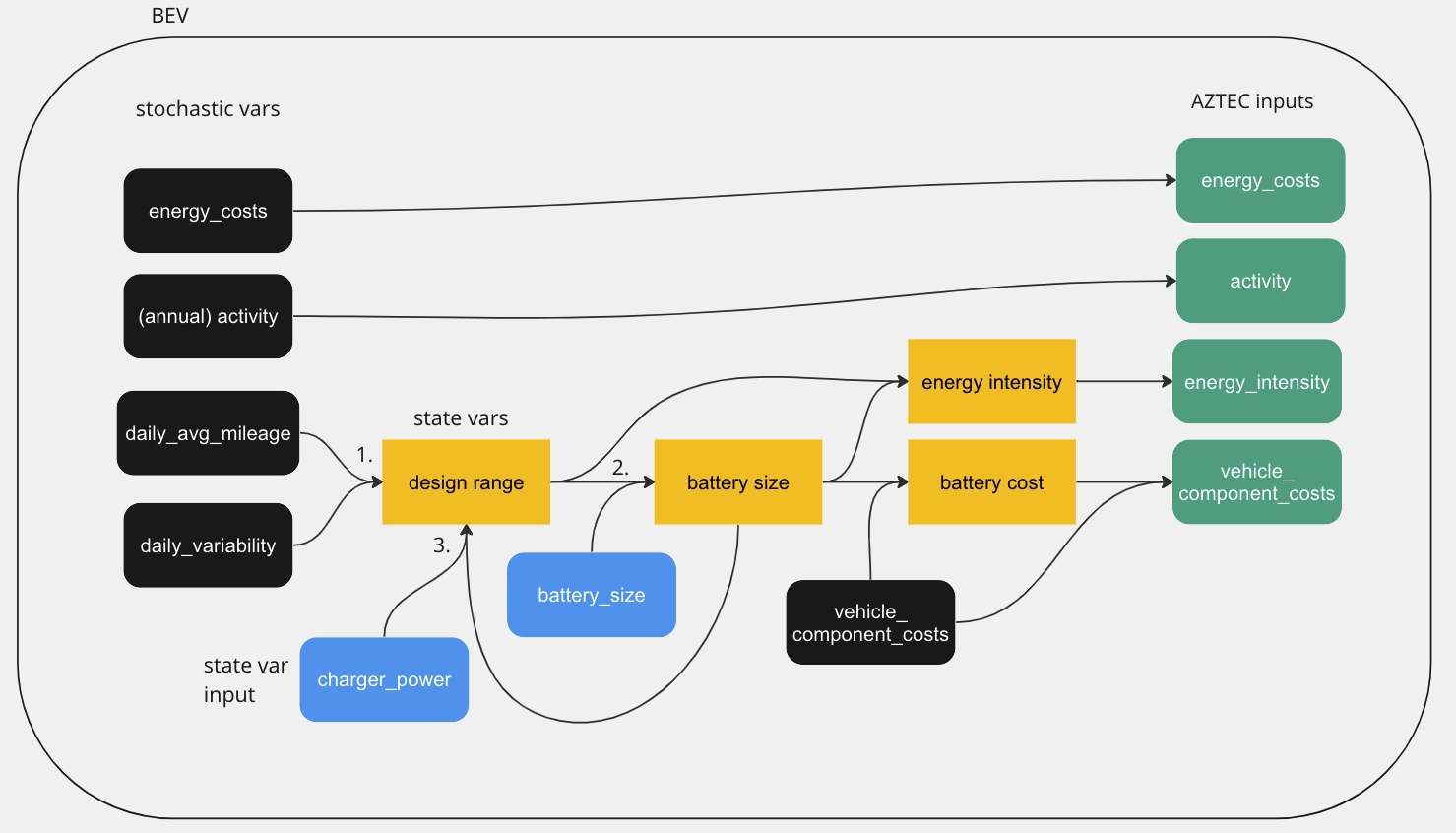 Figure 1: Sensitivity analysis flowchart for BEVs.
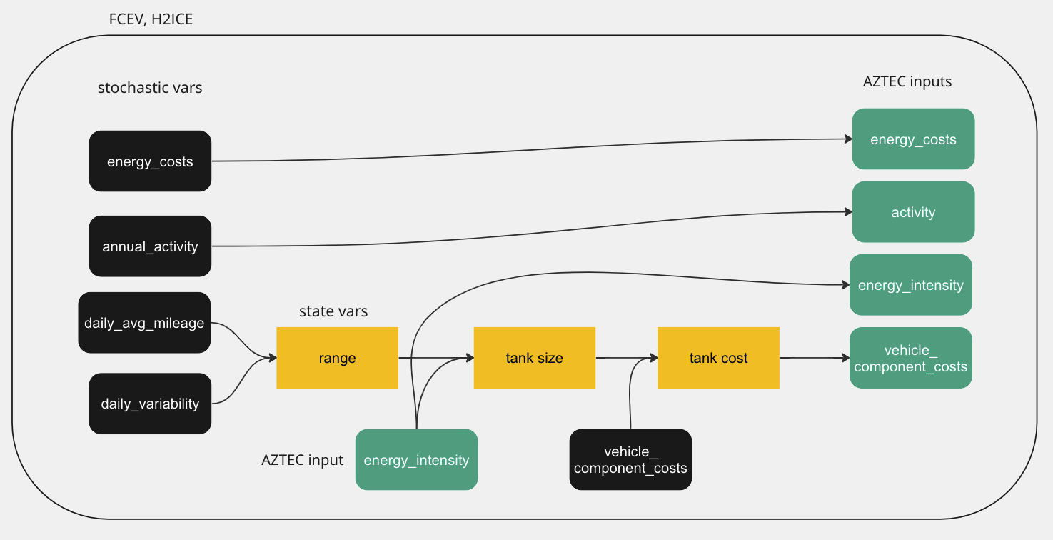 Figure 2: Sensitivity analysis flowchart for FCEVs and H2ICE vehicles.
Stochastic variable inputs
Stochastic variable inputs specify how the stochastic variables are varied between sensitivity scenarios. They contain all the same columns as the base input files, but instead of a “Value” column, they contain either:
- “Min”, “Max”, and “Step” columns, if the
sensitivity_typeis “sweep_range”, or - “DistType”, “Mean”, and “SD” columns, if the
sensitivity_typeis “sample_dist”.
Both the “Min” and “Max” will be included in the sweep, and the “Step” will be the increment between each value.
The “DistType” column specifies the probability distribution to sample from (either “normal” or “log-normal”), and the “Mean” and “SD” columns specify the mean and standard deviation of the (underlying) normal distribution.
Energy costs
- Description: Stochastic variable input file for the price of fuels (e.g., hydrogen, electricity, diesel)
- Corresponding AZTEC input: Energy costs
- Examples:
sensitivity/example/inputs/energy_costs_by_scen_sampled.csv,sensitivity/example/inputs/energy_costs_by_scen_swept.csv
Vehicle/component financing and costs
- Description: Stochastic variable input file for the price of vehicle components (e.g., battery, fuel cell, fuel tank)
- Corresponding AZTEC input: Vehicle/component financing and costs
- Example:
sensitivity/example/inputs/vehicle_component_costs_swept.csv
If “Battery” costs are given in “$/kWh”, the sensitivity module will calculate a battery price ($) as a state variable that depends on daily activity, battery range, and charging access.
Similarly, if “Hydrogen tank” costs are given in “$/kg”, the sensitivity module will calculate a hydrogen tank price ($) as a function of daily activity and energy intensity.
Otherwise, the sensitivity module will vary the cost of components directly.
Annual activity
- Description: Stochastic variable input file for annual activity (km), for emissions inventory
- Corresponding AZTEC input: Activity
- Examples:
sensitivity/example/inputs/activity_sampled.csv,sensitivity/example/inputs/activity_swept.csv
Daily average range
- Description: Stochastic variable input file for average daily range (km), for component size selection
- Corresponding AZTEC input: None
- Example:
sensitivity/example/inputs/daily_avg_range_swept.csv - Valid columns: Scenario, Region, Route, Vehicle, MY, Variable, Unit, [Min, Max, Step] or [DistType, Mean, SD]
The ‘Variable’ column should contain ‘DailyAvgRange’, and ‘Unit’ should be ‘km’.
This input should have values for each MY included in Vehicle/component financing and costs.
Daily variability
- Description: Stochastic variable input file for daily variability of activity (%), for component size selection
- Corresponding AZTEC input: None
- Example:
sensitivity/example/inputs/daily_variability_swept.csv - Valid columns: Scenario, Region, Route, Vehicle, MY, Variable, Unit, [Min, Max, Step] or [DistType, Mean, SD]
The ‘Variable’ column should contain ‘DailyVariability’, and ‘Unit’ should be ‘%’.
This input should have values for each MY included in Vehicle/component financing and costs.
State variable inputs
Battery size
- Description: BEV state variable input file for the range (km) of different battery sizes (kWh)
- Corresponding AZTEC input: None
- Example:
sensitivity/example/inputs/battery_size.csv - Valid columns: Scenario, Region, Route, Vehicle, Technology, MY, BatterySize, Range
This input is used to calculate the battery size required to meet the design range (as calculated by DesignRange = DailyAvgRange * (1 + DailyVariability)).
The model will choose the smallest capacity battery with a range greater than or equal to the design range.
This input should have values for each MY included in Vehicle/component financing and costs.
Charger power
- Description: BEV state variable input file for the most commonly available charging power (kW) and charging time (hr) by calendar year
- Corresponding AZTEC input: None
- Example:
sensitivity/example/inputs/battery_size.csv - Valid columns: Scenario, Region, Route, Vehicle, Technology, CY, ChargerPower, ChargerEfficiency, ChargingTime
If provided, this input is used to estimate the reduction in required battery size enabled by recharging during the day. This input triggers an iterative calculation, since a reduction in required range could result in a new battery size with a different efficiency, so we repeat the loop until the battery size converges. The default tolerance for convergence is 2%, and we allow no fewer than 5 and no more than 50 iterations. Regardless of available charger power and charging time, the model will not allow a battery size reduction that would result in a range less than 50% of the original design range.
The logic for updating the design range is given by: DesignRange' = DesignRange - EnergyFromCharging / VehicleEnergyIntensity
where EnergyFromCharging = ChargerPower * ChargerEfficiency * ChargingTime or BatterySize, whichever is smaller.
This input should have data for each CY listed as a MY in Vehicle/component financing and costs.
Outputs from sensitivity module
The sensitivity module will export the following files to the sensitivity_out_dir:
combined_config.ini: Combined configuration file with the sensitivity scenarios appended to the original AZTEC config fileactivity.csv: Annual activity values for each sensitivity scenarioenergy_costs.csv: Energy costs for each sensitivity scenarioenergy_intensity.csv: Energy intensity values for each sensitivity scenariovehicle_component_costs.csv: Vehicle/component costs for each sensitivity scenario
combined_config.ini is a valid AZTEC configuration file and will always be exported.
All the .csv files are valid AZTEC inputs, and will be exported as long as at least one upstream input they depend on is varied.
Users can feed these .csv outputs directly into the main AZTEC model via the combined_config.ini;
see Step-by-step sensitivity instructions for more details.
The sensitivity module will also export the following diagnostic outputs to sensitivity/diagnostic/ if diagnostic is set to True:
battery_size.csv: intermediate output showing the calculated battery size for each sensitivity scenariotank_size.csv: intermediate output showing the calculated tank size for each sensitivity scenario
Appendix
Retrofits
A scheme for modeling retrofits that alter operational parameters of the vehicle (e.g., emission factor, load factor, energy efficiency, etc.) is described below.
- Vehicles that will be retrofitted need to be separated out from vehicles that will not be retrofitted. In the “Vehicle” column in the base stock, these could be called “standard_AC” and “standard_AC_to_be_retrofitted”, e.g. They should have identical operational parameters.
- However, the vehicle service lifetime of the “standard_AC_to_be_retrofitted” should be decreased so that the vehicles “retire” at the time of the retrofit. Make sure that the depreciation schedule on these vehicles (and any components they contain) is sufficiently quick such that they have zero residual value (i.e., net depreciation = 100%) at the time of retirement (since they aren’t actually taken off the road or sold in the real world).
- In the input files, a new vehicle category called something like “standard_AC_with_retrofit” should be introduced, and it should have its stock projection set to the number of buses that will have been retrofitted in a given year (should start at zero if there are no retrofitted vehicles in the base fleet). Or, if a sales schedule is specified, the sales of “standard_AC_with_retrofit” would be used to define the times at which the “standard_AC_to_be_retrofitted” are retrofitted. Either way, the rate of introduction of “standard_AC_with_retrofit” should match the rate of retirement of “standard_AC_to_be_retrofitted”.
- The changes in operational parameters should be reflected in different values between “standard_AC_with_retrofit” and “standard_AC_to_be_retrofitted” in the relevant input files, like emission factors, load factor, energy efficiency, etc.
- The “standard_AC_with_retrofit” should have zero cost associated with vehicle components that are retained from the vehicle before the retrofit, e.g. vehicle body. Its only capital costs should be related to whatever component is installed as a retrofit.
- To get the TCO of retrofitted vehicles over their lifetime, the costs from the “standard_AC_to_be_retrofitted” and “standard_AC_with_retrofit” vehicle categories should be combined.